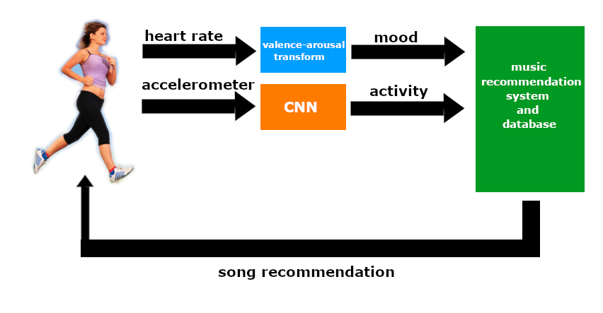
LOFI takes user inputs such as their mood, estimated using their heart rate variability, and their activity, estimated using a convolutional neural network, and recommends songs accordingly. The recommender algorithm implements an intuitive K-nearest neighbors algorithm to find songs “closest” to the user’s mood and activity in the latent valence-arousal-tempo space detailed below, returning the top K recommendations to the user by running the algorithm on a compact song metadata database on an app. In total, the system makes up a closed feedback loop where song recommendations that change a user’s mood can in turn change future recommendations.

Mood estimation

Representing mood in 2 dimensions: the valence-arousal space

One of the first questions that naturally surfaced when thinking up this project was, "How can you possibly quantify something like mood?"

In 1992, a paper was published that introduced a 2-dimensional, continuous representation of emotion in the Journal of Experimental Psychology [13]. This came to be known as the valence-arousal model of emotion (or, Circumplex Model of Affect), where different regions of the space represent different types of emotions.

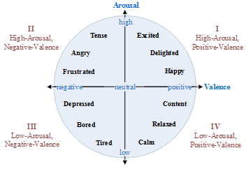
Valence, the horizontal axis, represents the positivity or negativity of an emotion. Arousal, the vertical axis, represents the energy of an emotion. For example, an emotion like happiness is characterized by high valence and high arousal, whereas anger is characterized by low valence and high arousal. This representation of emotion is desirable for our application since it is easy to visualize and to work with.

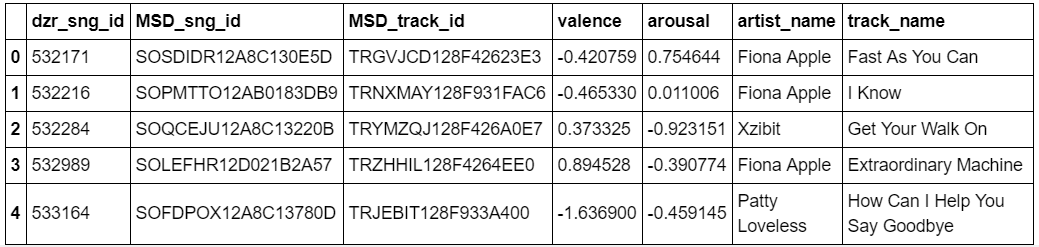
In 2018, researchers at Deezer, a music streaming service, published a paper on music mood classification [1a] and a dataset of songs embedded with their respective VA values [3]. By using a variety of techniques such as lyric semantic analysis, MFCC analysis (Mel frequency cepstral coefficients: what instruments and timbres were present) and crowdsourced tag analysis (mapping valence and arousal values to user tags of songs like "danceable" or "chill"), VA values for each song were algorithmically generated and standardized across the dataset.

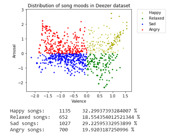
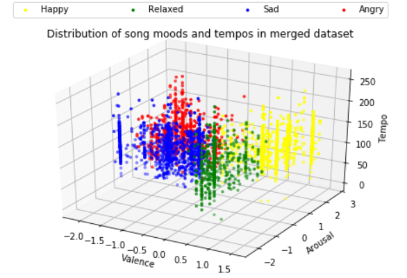
By dividing the valence-arousal space into 4 quadrants as per the paper on MoodyLyrics by Çano and Morisio [4a], the distribution of the Deezer dataset's distinction between 4 key "bins" of mood can be distinguished. Each data point plotted represents the valence and arousal value of a given song. Happy (yellow) songs are positive and high energy. Relaxed (green) songs are positive and low energy. Their respective complements are: sad (blue) songs that are negative with low energy, and angry (red) songs that are negative with high energy.

Signal processing of PPG signal

To calculate the HRV of the user, we analyzed the PPG signal measured by the Hexiwear. The PPG signal was measured over 5 seconds because the Hexiwear had limited local memory and its processor is relatively weak for our application. Hence, to keep the mood sent by the Hexiwear to be delivered within 45 seconds and not exceed Hexiwear’s memory, we had to limit the signal measurement period to 5 seconds.

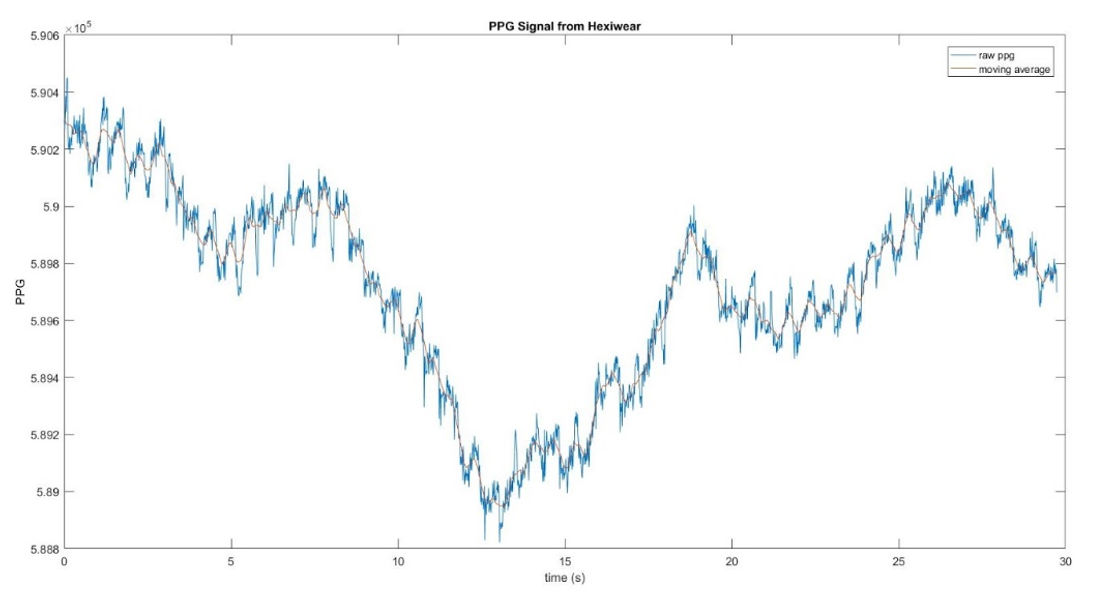
Since the PPG signal measured by the Hexiwear is very noisy, we needed to implement some algorithms to make the signal reasonably useable. So, we first subtracted the moving average of PPG signal from itself to normalize the signal. The below figure shows the plot of the raw PPG signal and its center moving average that has a window size of 25. Note that the below plots were taken over 30 seconds for better visualization of what our algorithm looks like.

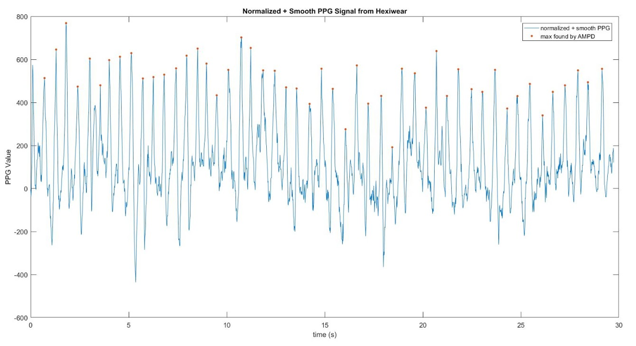
After normalizing the signal, we smoothed it out. To smooth it out, we set it equal to its moving average with a window size of 2. Using AMPD Algorithm as recommended in [16], we located the peaks as shown below. The window size for the AMPD Algorithm was chosen to be 25.

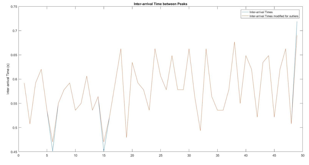
By inspection, the points determined to be local maximas by the algorithm are indeed maximas. Then, we find the time between each peak, and the below plot shows our derived inter-arrival times. Sometimes there are outliers though, and to control those, we set the outliers to be equal to some value.

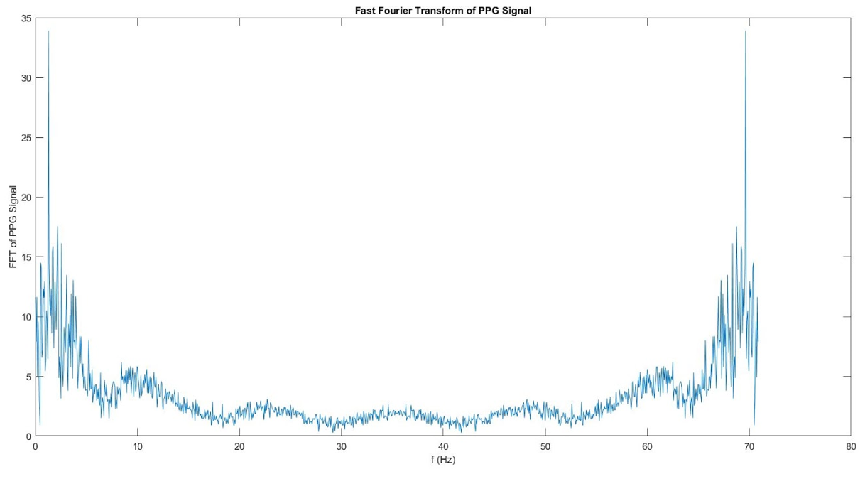
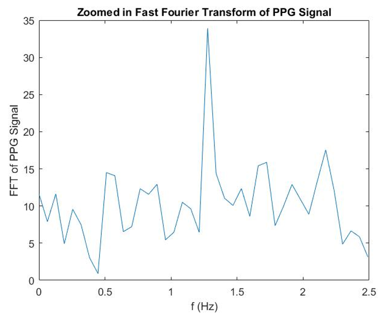
We use the inter-arrival times to calculate the SDNN. The formula for SDNN will be given later. To find HF and LF, we need to find the signal in its frequency domain. So, we found the Fast Fourier Transform (FFT) of the normalized and smoothed signal for best results. The plot below shows the FFT.

We are only interested in the frequency range from 0.04 Hz to 0.4 Hz for calculating HF and LF, so we zoomed the signal in to show the area of interest better. Below shows the zoomed in FFT.

Heart rate variability (HRV) and the VA space

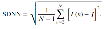
We found the HRV of the user by analyzing the PPG signal measured by the Hexiwear. Taking the inter-arrival times as I(n), we calculate SDNN by

(1)

Next, we calculate LF by integrating the FFT over the domain (0.04 Hz, 0.15 Hz) and then HF by integrating the FFT over the domain (0.15 Hz, 0.4 Hz). The calculation of LF/HF is trivial.

We take the first SDNN and LF/HF to map to the origin on the Valence/Arousal model. We then mapped the following HRV measurements to one of 25 points on the Valence/Arousal model. These 25 points are labeled below.

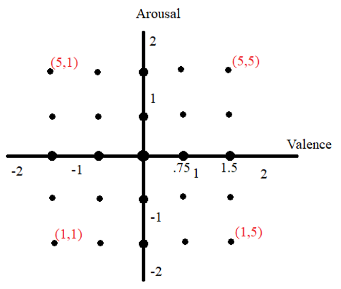
If change of SDNN is in some range, we mapped it to one of 5 specified valence values selected from {-1.5, -0.75, 0, 0.75, 1.5}. Similarly, the gain of LF/HF is mapped to 5 values of arousal. These ranges were estimated from the paper [14]. The red numbers are the encoded (Arousal, Valence) of the points. We chose to encode them to integer values from 1 to 5 for easier data transmission, since it’s unnecessary to send a float value.

Activity recognition

Goals of activity recognition

For this iteration of the project, the goal is to be able to distinguish between times when the user is active (i.e. jogging) or not active (i.e. studying or commuting). In the case of a user jogging, the system will aim to suggest music with a tempo matching their cadence as a priority, and matching mood is treated as secondary. Indeed, music recommended to the user depends on which of these two states they are in. In a more relaxed state, VA values of the song are the only factors in selecting song recommendations. But in a jogging state, where running to a song with a matching tempo makes more of an impact on the user's experience, song tempos are weighed more heavily.

To build on the aforementioned Deezer dataset with this in mind, we used the Million Songs dataset (MSD) [9] to lift the VA representation of songs to the 3rd dimension: tempo. Since the Deezer dataset was made from songs in the MSD, one of the dataset's fields was the MSD track ID. Using this field, songs in the Deezer set could be looked up in the MSD, where those songs have a variety of high-level feature information, one of such features being tempo. By appending this new column to the Deezer dataset, we can arrive at a 3D visualization of what we can now call VAT space (valence, arousal, tempo).

If time allows, and/or in future iterations of the project, more kinds of activities can be detected and songs can be suggested based on various other kinds of activities. The way is open for the project to be extended. Other features can be extracted from the MSD to add further dimensions to this latent space, or we could implement our own feature extraction algorithms to find features of interest.

Convolutional neural network (CNN) design and training

In order to infer what kind of activity a user is doing, convolutional neural networks (CNNs) were employed. Activity classification is most often done with CNNs or recurrent neural networks (RNNs). One of the main strengths of RNNs is their ability to use past information to make better inferences. This can shine in applications involving aperiodic time series data (such as in EEG data of subjects interacting with their environment). However, in the concise set of activities we wish to classify, the activities are either periodic (walking) or static (sitting). In such a case, taking windows of data (i.e., a number of samples of sensor data over a given time) can serve to be excellent predictors of the actual activity if the network was trained on such windows. Therefore, in an effort to keep the network model as simple (conceptually and in terms of number of parameters) as possible, a 1-dimensional CNN was chosen for the project.

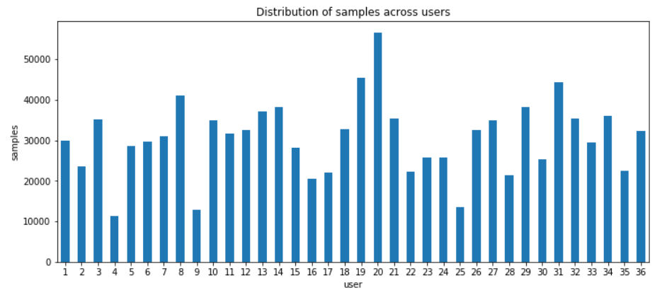
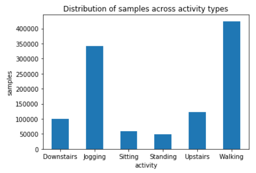
The dataset used to train the CNN was the Activity Prediction dataset from WISDM at Fordham University [5]. The dataset contains samples of 3D accelerometer data of a smartphone in the front leg pocket of several subjects, which matches the conditions that the project assumes most users would be in when using LOFI. The activities that the dataset consists of are:

• Sitting
• Standing
• Walking (on a flat surface)
• Walking upstairs
• Walking downstairs
• Jogging

The dataset was relatively evenly distributed across users (a good variety of different gaits and movement patterns across body types was acquired) and most of the activity samples were of either walking or jogging.

All of the data was sampled at 20 Hz. We normalized the acceleration values x during preprocessing across all samples according to equation (2).

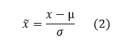
Here, x tilde is the normalized data, µ is the expected value of x, and σ is the standard deviation of x.

Before normalization, an accelerometer reading of magnitude 1 was equal to 1G, or 9.8 m/s squared. By optimizing over different window lengths and amounts of window overlap, we arrived at using a 3 second window with no overlap for training (60 samples per input to the network), validation, and testing of the data. Below are plots of a single window of different activities, preceded by a figure showing how the different smartphone acceleration axes were positioned relative to subjects' bodies during data collection [6].

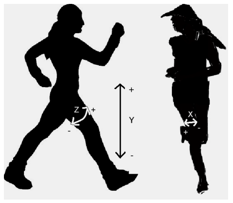
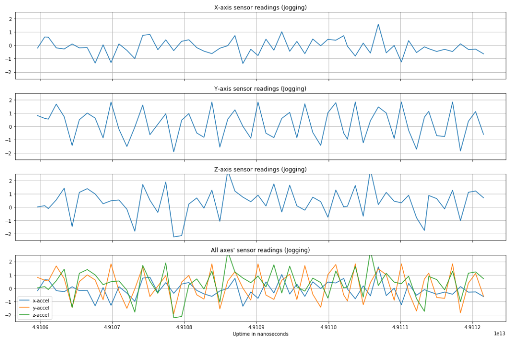
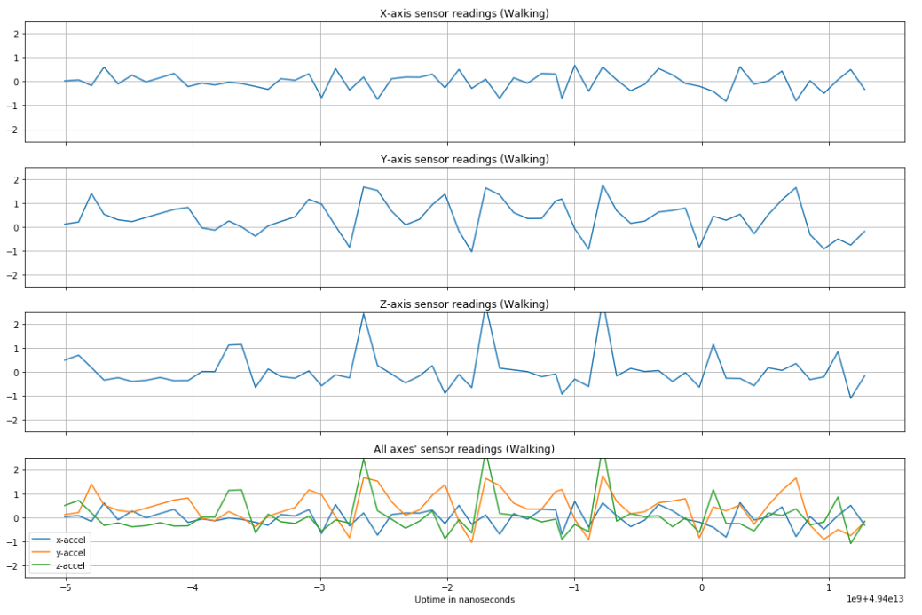
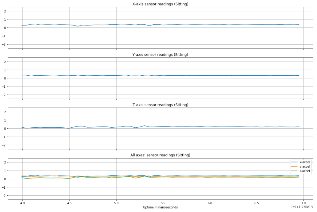
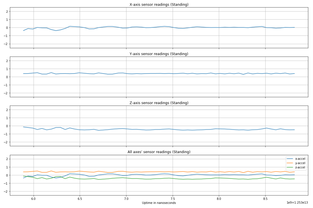
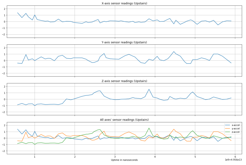
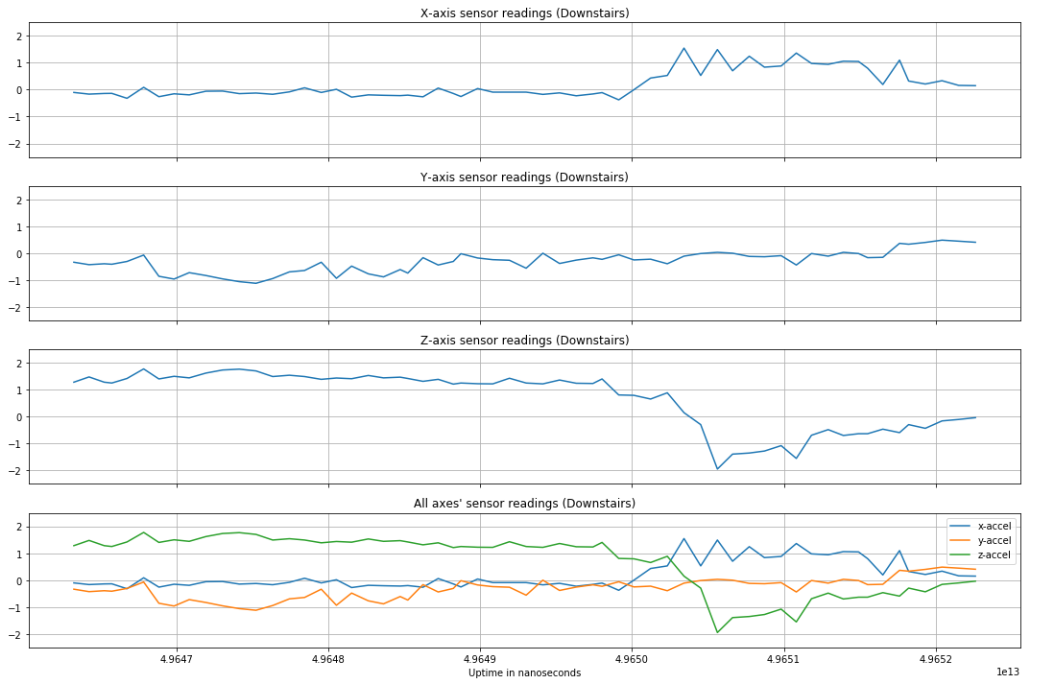
As expected, more vigorous activities like jogging have greater change in acceleration over time than a stationary activity like sitting. Other activities have observable, distinct features to set them apart from other types of activities (e.g. standing can be distinguished from sitting based on which axis feels gravity and walking up/downstairs have distinct "humps" in accelerometer readings).

The CNN architecture used is based off [7] and was visualized using Netron [8].

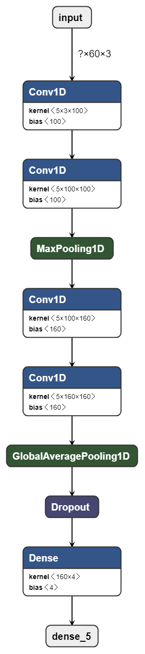
The convolution layers include a rectified linear unit (ReLU) at their output as their non-linear activation function. This popular choice of activation function is fast to compute and empirically performs well. The convolution filter size used was 4, and the number of filters in the first pair of convolution layers was 100, and in the second pair there were 160 filters used. Consecutive convolution layers allow for higher-level features in the sensor data to be discovered before being passed into the max pooling layer. These layers reduce intermediate tensor size while retaining the most critical information, all without adding extra training parameters. The dropout layer approximates bagging (bootstrap aggregating), a method of ensembling intended to improve generalization of the model. A dropout rate of 0.5 was used (half of the neurons would be "on"). Lastly, the output of the dropout layer is fed to a fully connected affine layer whose output is then fed to a softmax function to convert the scores into classification probabilities. The class (activity type) whose probability was the maximum among these was the activity the sample is to be classified as.

The Adam optimizer was used (with the Keras default learning rate and learning rate decay) since it has been found to often give strong empirical results as it utilizes both running means of momentum and past gradient history. A batch size of 400 samples was used in training the network over 10 epochs.

Stride rate estimation

A stride is a step, but is typically meant to potentially indicate a step longer than one would take while just walking - the term is common in, for example, runner subculture. Stride rate is defined as the number of times one's feet hit the ground as they move per unit time. We choose to focus on strides per minute due to the measure's resemblance to beats per minute, the unit of tempo used in music applications. Estimating the stride rate is important for the project since the stride rate provides us a way to recommend songs based on their tempo to provide as close a match as possible.

Stride rate is estimated by taking the average of 16 time differences between time-adjacent steps. In other words, every time a step is taken, a stride rate is estimated by dividing 60 by the time difference between the last step and the step that was just detected. 16 consecutive such measurements are averaged, and that effective stride rate is used to tempo-match with songs in the dataset. 16 steps was chosen due to its analogous relationship with 4 bars of music in 4/4, one of the most common time signatures; 4 bars of music (comprised of 16 quarter beats) is almost always indicative of a song's overall tempo and runners tend to want to synchronize their steps with the quarter beat of songs due to the importance and gravity of such beats in a musical context (they ground the song's strongest rhythms).

The step detector sensor in Android Studio was used to detect when steps are taken and the corresponding sensor event timestamps each step.

Song recommendation

K nearest neighbors for top recommendations

To take advantage of the VA space representation of the song dataset and HRV, we exploit the fact that listening to music with the same mood as a user is feeling has been shown to help the user feel better [11]. The top K songs are recommended to a user based on the Euclidean distance (norm 2) between a user's estimated mood in VA space and the K songs with the least distance to that mood. The K-nearest neighbors (KNN) algorithm is used to find these recommended songs.

Bringing it together: recommending based on mood (VA) and activity (tempo)

However, the desired minimum distance is a function of the user's activity - we want to recommend songs completely based on mood if a user is not active, but we want to factor in tempo if the user is active (and include some valence/arousal biases to avoid playing sad music during a workout). So, the top K recommendations are ultimately found by solving the following optimization problem for the smallest K distances:

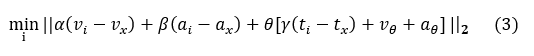
We wish to minimize the Euclidean distance of these quantities over all songs in the dataset i and return the K smallest distances and their respective songs. v, a, and t represent valence, arousal and tempo values, respectively. α, β, and γ are weights applied to their respective terms used for fine tuning recommendations. The subscript i refers to the values of one of the songs in the dataset. The subscript x refers to the values of a user’s mood (a user’s cadence when referring to tempo in t sub x). θ represents an indicator variable whose value can either be 1 or 0; θ = 1 if the user is active (jogging), else θ = 0. The subscript θ in the last term of the equation are the biases applied to the valence and arousal value regardless of user mood or song: if the user is jogging, we want to bias the valence and arousal of suggested songs such that songs that are too sad or relaxed are not suggested (an active workout would benefit from a higher-energy, positive playlist).

The user's activity state is classified as either active or non-active. The user state is used in determining how to weigh the song recommendation (3). At initialization, the user starts in the non-active state. "Active" activities include walking and jogging, and "non-active" activities include sitting and standing (more elaboration on this is provided in the Implementation section). If the user has 3 consecutive "active" activities classified, the user transitions to active state. If while in active state the user has 3 consecutive "non-active" activities classified, the user transitions to non-active state. The number of required consecutive classifications was determined from testing results as elaborated on in the Results section of the report.

Implementation

Translating everything to an app implementation

The project requires several components to implement. Heart rate measurements are taken by a Hexiwear module, which are then sent to a Raspberry Pi Zero W over Bluetooth Low Energy. Using PuTTY we could SSH into the Pi running Raspbian Lite and do everything we had to do over the command line. Key Python libraries used on the Pi were Cherrypy to host a webpage where encoded VA values would be posted to, and bluepy + bluez for handling BLE events. The Android Studio integrated development environment is used for app development, and the main development devices were an LG G5 and a Samsung Galaxy S3. The online MBed OS IDE was used to write and flash programs to the Hexiwear.

The online MBed OS IDE was the primary tool used to implement code written in C++ on the Hexiwear. Matlab was initially used to test out SDNN and LF/HF measurement algorithms, which were then rewritten in C++ for the Hexiwear to calculate them before sending VA estimates over BLE. The Pi receives these encoded VA estimates, and then writes them to a file that a concurrently-running Cherrypy script reads from to know what value to host on its website. The Pi is connected to a hotspot created by the smartphone and the app running on the same smartphone pulls this value from the website at the tap of a button. In the future, it would be ideal to remove the Pi as middleman of the system and have Hexiwear communicate directly to the smartphone. This design choice was made for ease of initial implementation.

To put the trained CNN onto the phone to be able to readily classify new accelerometer data, the TensorFlow Lite library was used. More precisely, the network was created and trained using the Keras Python library and was then converted to a .tflite model using a very handy .h5 to .tflite conversion script [19].

The dataset is included as a resource in the app and is cached at initialization of the program.

Apart from the MainActivity class of the app, classes were created for ActivityRecognizer, MusicRecommender, Song, StateMachine, and GetFromSite. Details of their implementation can be seen in the source code. Only a single activity was used in the app for ease of debugging and user operation, but asynchronous tasks were needed to implement the network features to read VA values from the Pi-hosted site.

Although prior analysis involved using a CNN to classify 6 different activities, the network actually implemented in the app is a 4-activity CNN classifying sitting, walking, jogging, and standing. The reason for this is that in our application, we would equate activities of walking, jogging, walking upstairs and walking downstairs to "active" activities (see more in the Results section) and therefore consider including walking upstairs/downstairs as redundant activities to classify for our purposes. In other words, we don't care about differentiating walking upstairs from downstairs from just walking on a flat surface for the purposes of this project: just knowing if the user is walking or jogging as opposed to staying still is informative enough for us to make appropriate music recommendations. Of course, building on this project to recommend music for more granularly defined types of activities can follow directly from the groundwork we laid out here.

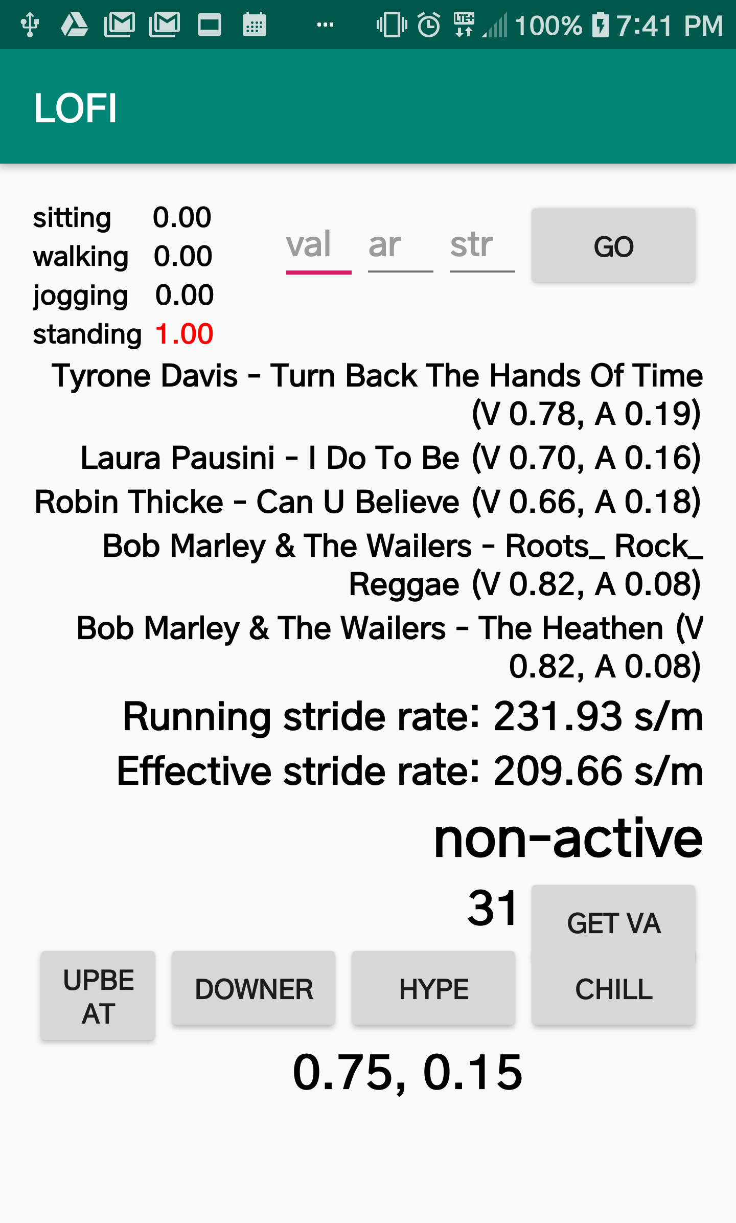
Depicted above is a screenshot of the interface. The upper-left corner shows the inferred probability of each of the 4 types of activities, and the classified activity has its probability colored red for easier identification. The upper-right corner contains manual entry fields for valence, arousal and stride rate values used for debugging. In practice, they are instead populated by valence, arousal, and stride rate data calculated as detailed earlier in the report.

The middle of the app is populated by the top K = 5 song recommendations based on the inputs given. In this example, since only valence and arousal was entered manually, the song recommendations are functions of only valence and arousal of songs. This can be confirmed by comparing the recommended songs' valence and arousal values with the inputted VA values. The app will recommend songs based on stride rate as well if the user is inferred to be doing an "active" activity (walking or jogging) for at least 3 consecutive activity inferences. Below the song recommendations are the running stride rate, which displays the most recent step-to-step stride rate estimation, and the effective stride rate which is the average of the last 16 step-to-step stride rates calculated. Below that is the activity level state that the app is operating in, determining the song recommendation scheme.

Below that is the encoded VA value next to the button the user can tap to read their current value from the Pi-hosted site ("GET VA"). Underneath are 4 manual adjustment buttons that the user can use to adjust the mood of songs initially recommended to them without having to rely completely on the VA estimates. Tapping the buttons changes the effective valence and arousal values used to recommend songs, which are shown as a pair at the bottom of the user interface. Tapping "Upbeat"/"Downer" increases/decreases valence by 0.05 and tapping "Hype/Chill" increases/decreases arousal by 0.05.

Optimization

Because the majority of the computing takes place on the smartphone, it was important to take reasonable measures to optimize performance. Additionally, the real-time nature of the system required constant and efficient computation as well as rendering of the results to the phone screen.

The merged dataset used for looking up songs originally included columns giving the Deezer song ID and the MSD song ID. By trimming these columns from the dataset, space was saved. Further improvements to saving space used by storing the dataset could come from enumerating the track IDs which are now a string of characters. By converting these to unique 32-bit integers, more space can be saved.

TensorFlow Lite is designed for optimized smartphone performance with practically unnoticeable differences in computations. This is accomplished through a variety of ways, e.g. quantization of values as well as disallowing double type variables and only allowing floats, among others. The package helps to minimize the memory needed to include such functions in the app as well as computation load. By choosing TensorFlow Lite instead of vanilla TensorFlow, the app performance has improved while still delivering consistent results.

Moving forward, some of the app code can be refactored to remove some redundancies and to make some components more generalizable to different numbers of parameters (such as making the number of activities to classify modular).