CNN performance

6-activity CNN performance on test data

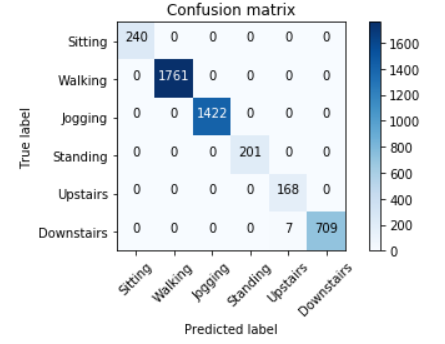
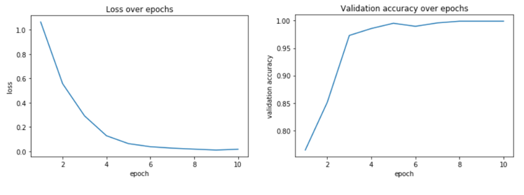
The sensor dataset was split into a 50-25-25 training-validation-test split. The testing accuracy achieved was 99.84%, which is an improvement over the best results of the paper that the dataset was created for [#], which had a 91.7% classification accuracy using a multilayer perceptron. Test samples were 3 second windows (60 samples) with no overlap of each of the 3 axes of accelerometer time series data. The test samples were randomly chosen across all activity types and all subjects, maximizing generalization performance of the network. Choosing a window size of 3 seconds and no overlap as hyperparameters along with the architecture choice made for a well-performing network, in theory. This could be owed to how relatively low-level features can be enough to distinguish between different activities, as discussed in the Design section. What mattered more was how the network would perform when implemented on a smartphone.

4-activity CNN performance on smartphone

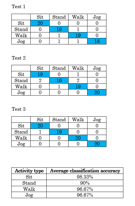
The network was implemented on the smartphone using the TensorFlow Lite library, as discussed more in Design. The reason for using a 4-activity network instead of the 6-activity one is also explained in Design. Each of the 3 tests consisted of each activity for 1 minute while the phone was in their front leg pocket. Since 3-second windows are taken as input to the network, there are 20 samples each minute and therefore each activity has 20 trials per test. A phone screen recording app [#] was used to record the classifications and review them.

For all experiments for this project, users walking walk at 2.5 mph and users jogging jog at 6 mph. This is measured either by an app or by the user moving on a treadmill whose speed can be set.

From the summary of classification accuracy at the bottom, even when implemented on the smartphone the network performs well. The activities walking and jogging have the highest classification accuracy as they are robust to different kinds of gaits and strides thanks to training over several test subjects. Interestingly, standing, one of the stationary activities, has the worst classification accuracy. This is due to the classification of standing being rather sensitive: one has to stand quite still, and upright to consistently be classified as standing. Leaning on a wall or even slight shifts in weight from one foot to the other can trigger misclassifications. Training can be augmented by introducing new standing samples complete with small variances included through leaning on surfaces and shifting weight around, or with feet re-positioning to make the network more robust.

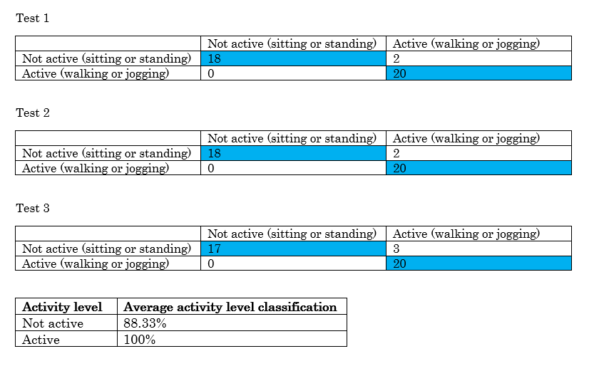
The last table’s 2nd column heading is meant to read “average activity level classification accuracy“.

The above experiment is meant to examine the network's performance in distinguishing between non-active activities (sitting, standing) and active activities (walking, jogging) so that the app may distinguish between operation modes: if the user is non-active, recommend songs based on mood only; otherwise, recommend songs based on stride rate as well. Each test is made up of 1 minute of classifications, so as before, 20 classifications per test. However, each of the tests were conducted back-to-back in a continuous 3-minute stretch. In the first minute (first test), at the 45 second mark the sitting user stood up and the walking user started to jog. 45 seconds later (30 seconds into test 2), the standing user sat down and the jogging user started to walk. This was repeated again 45 seconds later. These tests then capture classification performance during transition between activities as well.

While the network was always able to correctly classify active activities, it had some trouble correctly classifying non-active activities. Almost all of these inaccuracies (i.e. walking or jogging predicted when the user was sitting or standing) occurred during the transition period between sitting and standing: this change in gravity acting on the phone is sometimes understood as walking or jogging before "settling into" the transitioned-into activity within the next 3 classifications. While there is room for improvement in making transition detection more robust and prior work for it, for our project we find it sufficient to consider a user doing an active activity if their activity is classified as active for at least 3 consecutive classifications.

Stride rate estimation

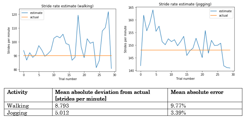
To conduct these tests, the smartphone was placed in the user's front leg pocket and in their free hand another smartphone accessed a website [#] that was used to estimate tempo by tapping a button repeatedly. As the user walked or jogged at a consistent stride rate, they tapped a button on the website at the same rate as their feet hitting the ground. The tempo estimated by the website, which estimates tempo identically to the smartphone implementation of stride rate estimation, is considered the ground truth. 30 effective stride rate estimations were captured for both walking and jogging. Again, walking was fixed at speed 2.5 mph and jogging at 6 mph.

Stride rate estimation is better for jogging than for walking. Jogging inherently produces a more pronounced step that is easier for the step detector to confidently detect. One reason that walking stride rate estimation tended to be higher than jogging is that sometimes during the test, the subject would turn around in place while at the end of the hall they walked down: this sudden increase in frequency of steps could have contributd to the error observed. The errors are relatively small and allow for recommending music based on stride rate as intended, still producing songs with a suitable tempo to jog to.

HRV estimation

We needed to know if our calculated SDNN and LF/HF were reasonable values. So, we compared our results with a paper measuring many measurements of HRV, two of which were SDNN and LF/HF. The below table shows the measurements from the research paper [17].

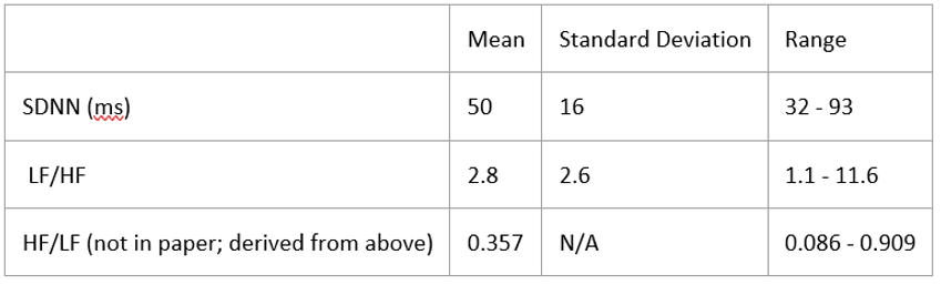
We compared this to our results:

We calculated HF/LF over a 30 second interval and got HF/LF = 0.763. Since our results are within the range of reasonable values, we determined that our results were acceptable.

Mood estimation

To test the reasonableness of our mood calculations, we tested it on a subject. This subject was not one of the authors to keep the results less biased. The subject had the Hexiwear on his index finger when measuring the PPG signal. The initial SDNN and LF/HF were calculated based on a 30 second measurement when the subject had no stimuli. Then, the subject’s SDNN and LF/HF were calculated based on the PPG taken when he was watching a sad video of animals almost dying. Film clips are used in research to elicit certain emotional responses, and research papers have found that pictures of animals dying are very effective in making subjects sad [18]. The PPG data when watching the sad video was split into two 15 sec intervals.

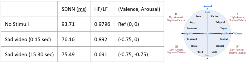
As you can see on the Valence/Arousal model, (-0.75, 0) and (-0.75, -0.75) map to the Depressed region. Hence, this shows that our algorithm is at least reasonable.

Song recommendation

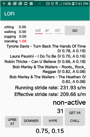
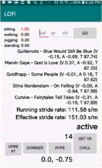
We recommended 5 songs based on valence, arousal, and cadence. If the user is detected in active mode, then song recommendations are weighted towards cadence, but valence and arousal are still considered. Below shows the recommendations in active mode.

If the user is detected in non-active mode, then the song recommendation is based solely on valence and arousal, since there is no cadence to be measured. Below shows the recommendations in non-active mode.